PREAMBLE (NOT PART OF THE STANDARD)

In order to promote public education and public safety, equal justice for all, a better informed citizenry, the rule of law, world trade and world peace, this legal document is hereby made available on a noncommercial basis, as it is the right of all humans to know and speak the laws that govern them.

END OF PREAMBLE (NOT PART OF THE STANDARD)

STANDARD METHODS: FOR THE EXAMINATION OF WATER AND WASTEWATER

18TH EDITION 1992

Prepared and published jointly by:
AMERICAN PUBLIC HEALTH ASSOCIATION
AMERICAN WATER WORKS ASSOCIATION
WATER ENVIRONMENT FEDERATION

Joint Editorial Board
Arnold E. Greenberg, APHA, Chairman
Lenore S. Clesceri, WEF
Andrew D. Eaton, AWWA

Managing Editor
Mary Ann H. Franson

Publication Office
American Public Health Association
1015 Fifteenth Street, NW
Washington, DC 20005

All rights reserved. No part of this publication may be reproduced, graphically or electronically, including entering in storage or retrieval systems, without the prior written permission of the publishers.

30M7/92

The Library of Congress has catalogued this work as follows:
American Public Health Association.
      Standard methods for the examination of water and wastewater.
ISBN 0-87553-207-1

Printed and bound in the United States of America.
     Composition: EPS Group, Inc., Hanover, Maryland
          Set in: Times Roman
     Printing: Victor Graphics, Inc., Baltimore, Maryland
     Binding: American Trade Bindery, Baltimore, Maryland
     Cover Design: DR Pollard and Associates, Inc., Arlington, Virginia

2510 CONDUCTIVITY^*

2510 A. Introduction

Conductivity, k, is a measure of the ability of an aqueous solution to carry an electric current. This ability depends on the presence of ions; on their total concentration, mobility, and valence; and on the temperature of measurement. Solutions of most inorganic compounds are relatively good conductors. Conversely, molecules of organic compounds that do not dissociate in aqueous solution conduct a current very poorly, if at all.

1. Definitions and Units of Expression

Conductance, G, is defined as the reciprocal of resistance, R:

where the unit of R is ohm and G is ohm⁻¹ (sometimes written mho). Conductance of a solution is measured between two spatially fixed and chemically inert electrodes. To avoid polarization at the electrode surfaces the conductance measurement is made with an alternating current signal.¹ The conductance of a solution, G, is directly proportional to the electrode surface area, A, cm², and inversely proportional to the distance between the electrodes, L. cm. The constant of proportionality, k, such that:

is called “conductivity” (preferred to “specific conductance”). It is a characteristic property of the solution between the electrodes. The units of k are 1/ohm-cm or mho per centimeter. Conductivity is customarily reported in micromhos per centimeter. Conductivity is customarily reported in micromhos per centimeter (μmho/cm).

In the International System of Units (SI) the reciprocal of the ohm is the siemens (S) and conductivity is reported as millisiemens per meter (mS/m); 1 mS/m = 10 μmhos/cm and 1 μS/cm = 1 μmho/cm. To report results in SI units of mS/m divide μmhos/cm by 10.

To compare conductivities, values of k are reported relative to electrodes with A = 1 cm² and L = 1 cm. Absolute conductances, G_s, of standard potassium chloride solutions between electrodes of precise geometry have been measured; the corresponding standard conductivities, k_s, are shown in Table 2510:I.

The equivalent conductivity, A, of a solution is the conductivity per unit of concentration. As the concentration is decreased toward zero, A approaches a constant, designated as A^°. With k in units of micromhos per centimeter it is necessary to convert concentration to units of equivalents per cubic centimeter; therefore:

A = 0.001k/concentration

where the units of A, k, and concentration are mho-cm²/equivalent, μmho/cm, and equivalent/L, respectively. Equivalent conductivity,

A, values for several concentrations of KCI are listed in Table 2510:I.

2. Measurement

a. Instrumental measurements: In the laboratory, conductance, G_s, (or resistance) of a standard KCI solution is measured and from the corresponding conductivity, k_s, (Table 2510:I) a cell constant, C, cm⁻¹, is calculated:

Most conductivity meters do not display the actual solution conductance, G, or resistance, R; rather, they generally have a dial that permits the user to adjust the internal cell constant to match the conductivity, k_s, of a standard. Once the cell constant has been determined, or set, the conductivity of an unknown solution,

k_u = CG_u

will be displayed by the meter.

Distilled water produced in a laboratory generally has a conductivity in the range 0.5 to 3 μmhos/cm. The conductivity increases shortly after exposure to both air and the water container.

The conductivity of potable waters in the United States ranges generally from 50 to 1500 μmhos/cm. The conductivity of domestic wastewaters may be near that of the local water supply, although some industrial wastes have conductivities above 10 000 μmhos/cm. Conductivity instruments are used in pipelines, channels, flowing streams, and lakes and can be incorporated in multiple-parameter monitoring stations using recorders.

^* Approved by Standard Methods Committee. 1991

Most problems in obtaining good data with conductivity monitoring equipment are related to electrode fouling and to inadequate sample circulation. Conductivities greater than 10 000 to 50 000 μmho/cm or less than about 10 μmho/cm may be difficult to measure with usual measurement electronics and cell capacitance. Consult the instrument manufacturer’s manual or published references.^1,5,6

Laboratory conductivity measurements are used to:

• Establish degree of mineralization to assess the effect of the total concentration of ions on chemical equilibria, physiological effect on plants or animals, corrosion rates, etc.

• Assess degree of mineralization of distilled and deionized water.

• Evaluate variations in dissolved mineral concentration of raw water or wastewater. Minor seasonal variations found in reservoir waters contrast sharply with the daily fluctuations in some polluted river waters. Wastewater containing significant trade wastes also may show a considerable daily variation.

• Estimate sample size to be used for common chemical determinations and to check results of a chemical analysis.

• Determine amount of ionic reagent needed in certain precipitation and neutralization reactions, the end point being denoted by a change in slope of the curve resulting from plotting conductivity against buret readings.

• Estimate total dissolved solids (mg/L) in a sample by multiplying conductivity (in micromhos per centimeter) by an empirical factor. This factor may vary from 0.55 to 0.9, depending on the soluble components of the water and on the temperature of measurement. Relatively high factors may be required for saline or boiler waters, whereas lower factors may apply where considerable hydroxide or free acid is present. Even though sample evaporation results in the change of bicarbonate to carbonate the empirical factor is derived for a comparatively constant water supply by dividing dissolved solids by conductivity.

• Approximate the milliequivalents per liter of either cations or anions in some waters by multiplying conductivity in units of micromhos per centimeter by 0.01.

b. Calculation of conductivity: For naturally occurring waters that contain mostly Ca²⁺, Mg²⁺, Na⁺, K⁺, HCO₃⁻, SO₄²⁻, and Cl⁻ and with TDS less than about 2500 mg/L, the following procedure can be used to calculate conductivity from measured ionic concentrations.⁷ The abbreviated water analysis in Table 2510:II illustrates the calculation procedure.

At infinite dilution the contribution to conductivity by different kinds of ions is additive. In general, the relative contribution of each cation and anion is calculated by multiplying equivalent conductances. λ^°₊ and λ^°₋, mho-cm²/equivalent, by concentration

in equivalents per liter and correcting units. Table 2510:III contains a short list of equivalent conductances for ions commonly found in natural waters.⁸ Trace concentrations of ions generally make negligible contribution to the overall conductivity. A temperature coefficient of 0.02/deg is applicable to all ions, except H⁺ (0.0139/deg) and OH⁻ (0.018/deg).

At finite concentrations, as opposed to infinite dilution, conductivity per equivalent decreases with increasing concentration (see Table 2510:I). For solutions composed of one anion type and one cation type, e.g., KCl as in Table 2510:I, the decrease in conductivity per equivalent with concentration can be calculated, ± 0.1%, using an ionic-strength-based theory of Onsager.⁹ When mixed salts are present, as is nearly always the case with natural and wastewaters, the theory is quite complicated.¹⁰ The following semiempirical procedure can be used to calculate conductivity for naturally occurring waters:

First, calculate infinite dilution conductivity (Table 2510:II, Column 4):

k^° = ∑|z_i|(λ°_−i)(mM_i) + ∑|z_i|(λ°_−i)(mM_i)

where:

            |z_i| = absolute value of the charge of the i-th ion,
         mM_i = millimolar concentration of the i-th ion, and
λ°_−i, λ°_−i = equivalent conductance of the i-th ion.

If mM is used to express concentration, the product, (λ°₊) (mM_i) or (λ°₋)(mM_i), corrects the units from liters to cm³. In this case k° is 578.2 μmho/cm (Table 2510:II, Column 4).

Next, calculate ionic strength, IS in molar units:

IS = ∑z²₁(mM₁)/2000

The ionic strength is 15.33/2000 = 0.00767 M (Table 2510:II, Column 5).

Calculate the monovalent ion activity coefficient, y using the Davies equation for IS ≤ 0.5 M and for temperatures from 20 to 30°C.^9.11

y = 10^{−0.5 [IS1/2/(1 + IS1/2) − 0.3IS]}

In the present example IS = 0.00767 M and y = 0.91.

Finally, obtain the calculated value of conductivity, k_calc, from:

k_calc = k°y²

In the example being considered, k_calc = 578.2 × 0.91² = 478.8 μmho/cm versus the reported value as measured by the USGS of 477 μmho/cm.

For 39 analyses of naturally occurring waters, ^7,12 conductivities calculated in this manner agreed with the measured values to within 2%.

3. References

1. WILLARD. H.H., L.L. MERRITT & J.A. DEAN. 1974. Instrumental Methods of Analysis, 5th ed. D. Van Nostrand Company, New York, N. Y.
2. WU. Y.C., W.F. KOCH, W.J. HAMER & R.L. KAY. 1987. Review of electrolytic conductance standards. J. Solution Chem. 16:No.12.
3. JASPER, W.S. 1988. Secondary Standard Potassium Chloride Conductivity Solutions at 25°C. Corporate Metrology Laboratory. YSI Inc., Yellow Springs, Ohio.
4. ORGANISATION INTERNATIONALE DE METROLOGIE LEGALE. 1981. Standard Solutions Reproducing the Conductivity of Electrolytes, International Recommendation No. 56, 1st ed., June 1980. Bur. International de Métrologie Légale, Paris, France.
5. AMERICAN SOCIETY FOR TESTING AND MATERIALS. 1982. Standard test methods for electrical conductivity and resistivity of water. ASTM Designation D1125-82.
6. SCHOEMAKER, D.S., C.W. GARLAND & J.W. NIBLER. 1989. Experiments in Physical Chemistry. 5th ed. McGraw–Hill Book Co., New York, N. Y.
7. HAMILTON, C.E. 1978. Manual on Water. ASTM Spec. Tech. Publ. 442A, 4th ed. American Soc. Testing & Materials. Philadelphia, Pa.
8. DEAN, J.A. 1985. Lange’s Handbook of Chemistry, 13th ed. McGraw–Hill Book Co., New York. N.Y.
9. ROBINSON, R.A. & R.H. STOKES. 1959. Electrolyte Solutions. 2nd ed. Academic Press, New York, N. Y.
10. HARNED, H.S. & B.B. OWEN. 1958. The Physical Chemistry of Electrolytic Solutions. 3rd ed. Reinhold Publishing Corp., New York. N.Y.
11. DAVIES, C. W. 1962. Ion Association. Elsevier Press, Amsterdam. The Netherlands.
12. TCHOBANOGLOUS, G. & E.D. SCHROEDER. 1985. Water Quality. Vol. 1. Addison–Wesley Publishing Company, Reading, Mass.

2510 B. Laboratory Method

1. General Discussion

See Section 2510A.

2. Apparatus

a. Self-contained conductivity instruments: Use an instrument capable of measuring conductivity with an error not exceeding 1‰ or 1 µmho/cm. Whichever is greater.

b. Thermometer, capable of being read to the nearest 0.1°C and covering the range 23 to 27°C. Many conductivity meters are equipped to read an automatic temperature sensor.

c. Conductivity cell:

1) Platinum-electrode type—Conductivity cells containing platinized electrodes are available in either pipet or immersion form. Cell choice depends on expected range of conductivity. Experimentally check instrument by comparing instrumental results with true conductivities of the KCI solutions listed in Table 2510:I. Clean new cells, not already coated and ready for use, with chromic-sulfuric acid cleaning mixture and platinize the electrodes before use. Subsequently, clean and replatinize them whenever the readings become erratic, when a sharp end point cannot be obtained, or when inspection shows that any platinum black has flaked off. To platinize, prepare a solution of 1 g chloroplatinic acid, H₂PtCl₆·6H₂O, and 12 mg lead acetate in 100 mL distilled water. A more concentrated solution reduces the time required to platinize electrodes and may be used when time is a factor, e.g., when the cell constant is 1.0/cm or more. Immerse electrodes in this solution and connect both to the negative terminal of a 1.5–V dry cell battery. Connect positive side of battery to a piece of platinum wire and dip wire into the solution. Use a current such that only a small quantity of gas is evolved. Continue electrolysis until both cell electrodes are coated with platinum black. Save platinizing solution for subsequent use. Rinse electrodes thoroughly and when not in use keep immersed in distilled water.

2) Nonplatinum-electrode type—Use conductivity cells containing electrodes constructed from durable common metals (stainless steel among others) for continuous monitoring and field studies. Calibrate such cells by comparing sample conductivity with results obtained with a laboratory instrument. Use properly designed and mated cell and instrument to minimize errors in cell constant.

3. Reagents

a. Conductivity water: Any of several methods can be used to prepare reagent–grade water. The methods discussed in Section 1080 are recommended. The conductivity should be small compared to the value being measured.

b. Standard potassium chloride solution, KCl, 0.0100M: Dissolve 745.6 mg anhydrous KCl in conductivity water and dilute to 1000 mL in a class A volumetric flask at 25°C. This is the standard reference solution, which at 25°C has a conductivity of 1412 µmhos/cm. It is satisfactory for most samples when the cell has a constant between 1 and 2 cm⁻¹. For other cell constants, use stronger or weaker KCl solutions listed in Table 2510:1. Store in a glass–stoppered borosilicate glass bottle.

4. Procedure

a. Determination of cell constant: Rinse conductivity cell with at least three portions of 0.01M KCl solution. Adjust temperature of a fourth portion to 25.0 ± 0.1°C. If a conductivity meter displays resistance, R ohms, measure resistance of this portion and note temperature. Compute cell constant. C:

C(cm⁻¹) = (0.001 412)(R_KCL)[1 + 0.019(t − 25)]

Where:

  R_KCL = measured resistance, ohms, and
      t = observed temperature, °C.

Conductivity meters often indicate conductivity directly. Commercial probes commonly contain a temperature sensor. With such instruments, rinse probe three times with 0.0100M KCI, as above. Adjust temperature compensation dial to 0.0191 C = ⁻¹. With probe in standard KCI solution, adjust meter to read 1412 µmho/cm. This procedure automatically adjusts cell constant internal to the meter.

b. Conductivity measurement: Rinse cell with one or more portions of sample. Adjust temperature of a final portion to about 25°C. Measure sample resistance or conductivity and note temperature to ±0.1°C.

5. Calculation

The temperature coefficient of most waters is only approximately the same as that of standard KCI solution; the more the temperature of measurement deviates from 25.0°C, the greater the uncertainty in applying the temperature correction. Report all conductivities at 25.0°C.

a. When sample resistance is measured, conductivity at 25°C is:

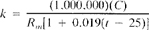
where:

      k = conductivity, µmhos/cm,
     C = cell constant, cm¹,
   R_m = measured resistance of sample, ohms, and
      t = temperature of measurement.

b. When sample conductivity is measured without internal temperature compensation conductivity at 25°C is:

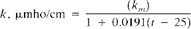
where:

      k_m = measured conductivity in units of µmho/cm at t°C, and other units are defined as above.

For instruments with automatic temperature compensation and readout directly in μmho/cm or similar units, the readout automatically is corrected to 25.0°C. Report displayed conductivity in designated units.

c. For instruments giving values in SI units,

1 mS/m = 10 µmhos/cm, or conversely,
1 µmho/cm = 0.1 mS/m.

6. Precision and Bias

The precision of commercial conductivity meters is commonly between 0.1 and 1.0.‰ Reproducibility of 1 to 2% is expected after an instrument has been calibrated with such data as is shown in Table 2510:I.