This library of books, audio, video, and other materials from and about India is curated and maintained by Public Resource. The purpose of this library is to assist the students and the lifelong learners of India in their pursuit of an education so that they may better their status and their opportunities and to secure for themselves and for others justice, social, economic and political.
This item has been posted for non-commercial purposes and facilitates fair dealing usage of academic and research materials for private use including research, for criticism and review of the work or of other works and reproduction by teachers and students in the course of instruction. Many of these materials are either unavailable or inaccessible in libraries in India, especially in some of the poorer states and this collection seeks to fill a major gap that exists in access to knowledge.
For other collections we curate and more information, please visit the Bharat Ek Khoj page. Jai Gyan!
IRC : 64-1990
(First Revision)
Published by
THE INDIAN ROADS CONGRESS
Jamnagar House, Shahjahan Road,
New Delhi-110011
1990
Price Rs. 80/-
(Plus Packing & Postage)
GUIDELINES FOR CAPACITY OF ROADS IN RURAL AREAS
Capacity analysis is fundamental to the planning, design and operation of roads, and provides, among other things, the basis for determining the carriageway width to be provided at any point in a road network with respect to the volume and composition of traffic. Moreover, it is a valuable tool for evaluation of the investments needed for future road construction and improvements, and for working out priorities between the competing projects.
"Tentative Guidelines on Capacity of Roads in Rural Areas" were published by the Indian Roads Congress in 1976 (IRC : 64-1976). Since then some basic research on this topic has been carried out in the country, notably through the Road User Cost Study, in which experiments were conducted to measure free speeds, and speed-flow relationships at a series of sites under typical Indian traffic condition. This has led to a better understanding of the speed and volume characteristics on roads of different pavement widths and types under various conditions.
Based on findings from the above studies, as well as current practices in other countries, it has been possible to revise the Tentative Guidelines published earlier and place them on a more firm footing. At the same time, it is recognised that as a result of additional data coming through, especially under the Traffic Simulation Studies currently in progress, the capacity standards may need further modification in due course.
These guidelines were considered by the Traffic Engineering Committee (personnel given below) in their meeting held at New Delhi on the 27th March, 1990.
| R.P. Sikka | ... | Convenor |
| M.K. Bhalla | ... | Member-Secretary1 |
| V.K. Arora | S.K. Sheriff | |
| P.S. Bawa | S.K. Sikdar | |
| Dilip Bhattacharya | Dr. M S. Srinivasan | |
| A.G. Borkar | H.C. Sethi | |
| Dr. S. Raghava Chari | Surjit Singh | |
| Prof. Dinesh Mohan | P.G. Valsankar | |
| Dr. A.K. Gupta | S. Vishwanath | |
| R.G. Gupta | Director, HRS, Madras | |
|
V.P. Kamdar J.B. Mathur N.P. Mathur S.K. Mukherjee S.M. Parulkar S.M. Parulkar Dr. S.P. Palaniswamy Prof. N. Ranganathan Dr. A.C. Sarńa D. Sanyal |
Director, Transport Research (MOST) (R.C. Sharma) Deputy Commissioner (Traffic), Delhi The President, IRC (V.P. Kamdar) — Ex-officio The DG (RD) (K.K. Sarin) — Ex-officio The Secretary, IRC (D.P. Gupta) — Ex-officio |
|
| Corresponding Members | ||
| T. Ghosh | The Executive Director, ASRTU New Delhi | |
| N.V. Merani | The Chief Engineer (NH) Kerala P.W.D., (S.Kesvan Nair) |
|
| Prof. M.S.V. Rao | ||
These were processed by the Highways Specifications and Standards Committee in their meeting held on 16th April 1990, subject to certain modifications which were subsequently carried out by the Convenor and Member-Secretary of the Committee. These guidelines were then approved by the Executive Committee and later by the Council for publication in their meeting held on 20th March and 29th April 1990, respectively.2
The guidelines contained in this publication are applicable to long stretches of rural highways as presently existing in the country. For this the rural highways are considered as all-purpose roads, with no control of access, and with heterogeneous mix of fast and slow-moving vehicles.
The capacity values recommended further on apply in general to those sections which have neither the restraints of narrow structures nor any deficiencies of visibility or other geometric features like curves. Moreover, the norms indicated are meant to be used only when a nominal amount of animal-drawn vehicles (say upto 5 per cent) is present in the traffic stream during the peak hour, which is generally the case on rural highways.
The guidelines are not applicable to the design of intersections on rural highways. The capacity of these intersections will have to be determined individually. The guidelines are also not applicable to urban roads and streets.
Further, the capacity of access-controlled roads, such as expressways, is outside the purview of these guidelines.
An understanding of concept of highway capacity is facilitated through a clear definition of certain terms.
Speed is the rate of motion of individual vehicles or of a traffic stream. It is measured in metres per second, or more generally as kilometres per hour. Two types of speed measurements are commonly used in traffic flow analysis; viz. (i) Time mean speed and (ii) Space mean speed. For the purpose of these guidelines, the speed measure used is "Space mean speed"
Time Mean Speed is the mean speed of vehicles observed at a point on the road over a period of time. It is the mean spot speed.
Space Mean Speed is the mean speed of vehicles in a traffic stream at any instant of time over a certain length (space) of road. In other words, this is average speed based on the average travel time of vehicles to traverse a known segment of roadway. It is slightly less in value than the time mean speed.3
Volume (or flow) is the number of vehicles that pass through a given point on the road during a designated time interval. Since roads have a certain width and a number of a lanes are accommodated in that width, flow is always expressed in relation to the given width (i.e. per lane or per two lanes etc.). The time unit selected is an hour or a day. ADT is the volume of Average Daily Traffic when measurements are taken for a few days. AADT is the Annual Average Daily Traffic when measurements are taken for 365 days of the year and averaged out.
Density (or concentration) is the number of vehicles occupying a unit length of road at an instant of time. The unit length is generally one kilometre. Density is expressed in relation to the width of the road (i.e. per lane or per two lanes etc.) When vehicles are in a jammed condition, the density is maximum. It is then termed as the jamming density.
Capacity is defined as the maximum hourly volume (Vehicles per hour) at which vehicles can reasonably be expected to traverse a point or uniform section of a lane or roadway during a given time period under the prevailing roadway, traffic and control conditions.
Design Service Volume is defined as the maximum hourly volume at which vehicles can reasonably be expected to traverse a point or uniform section of a lane or roadway during a given time period under the prevailing roadway, traffic and control conditions while maintaining a designated level of service.
Peak-Hour Factor is defined as the traffic volume during peak hour expressed as a percentage of the AADT. The peak hour volume in this case is taken as the Thirtieth Hourly Volume (i.e. the volume of traffic which is exceeded only during 30 hours in a year).
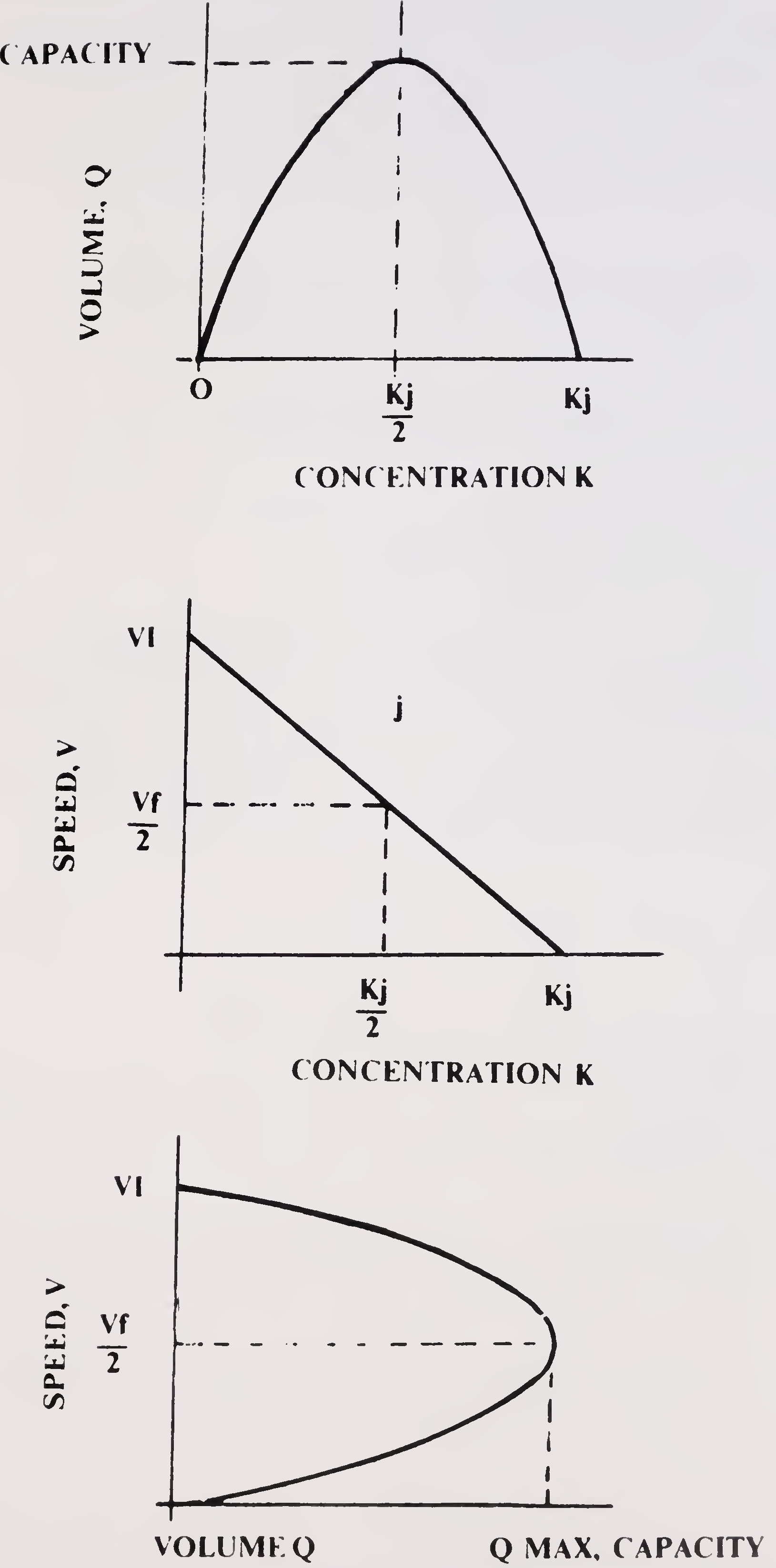
The idealised relationship between speed, volume and density is expressed in the three basic diagrams given in Fig. 1 which are collectively known as the Fundamental Diagram of Traffic Flow.4
Fig. 1. Fundamental diagram of traffic flow5
It will be seen that the speed-density relationship is a straight line, having maximum speed (free speed) when traffic is low and having zero speed when vehicles are jammed.
The speed-volume relationship is a parabola, having maximum volume at a value of speed equal to half the free speed.
The density-volume relationship is a parabola, having a maximum volume at a value of density equal to half the jamming density.
The following relationship exists :
| where | Q | = | K.V |
| Q | = | Volume | |
| K | = | Density, and | |
| V | = | Speed |
Maximum volume that can be accommodated on the road (Qmax, or vehicles per unit time) is considered to be the road capacity. From the idealised relationship shown in Fig. 1, it can be seen that the maximum volume occurs at half the free speed and half the jamming densitv, meaning thereby that:

Level of Service is defined as a qualitative measure describing operational conditions within a traffic stream, and their perception by drivers /passengers.
Level of Service definition generally describes these conditions in terms of factors such as speed and travel time, freedom to manoeuvre, traffic interruptions, comfort, convenience and safety. Six levels of service are recognised commonly, designated from A to F, with Level of Service A representing the best operating condition (i.e. free flow) and level of service F the worst (i.e. forced or break-down flow).
Fig. 2. shows the various levels of service in the form of indicative volume-flow conditions. Each of the levels can be generally described as follows :6
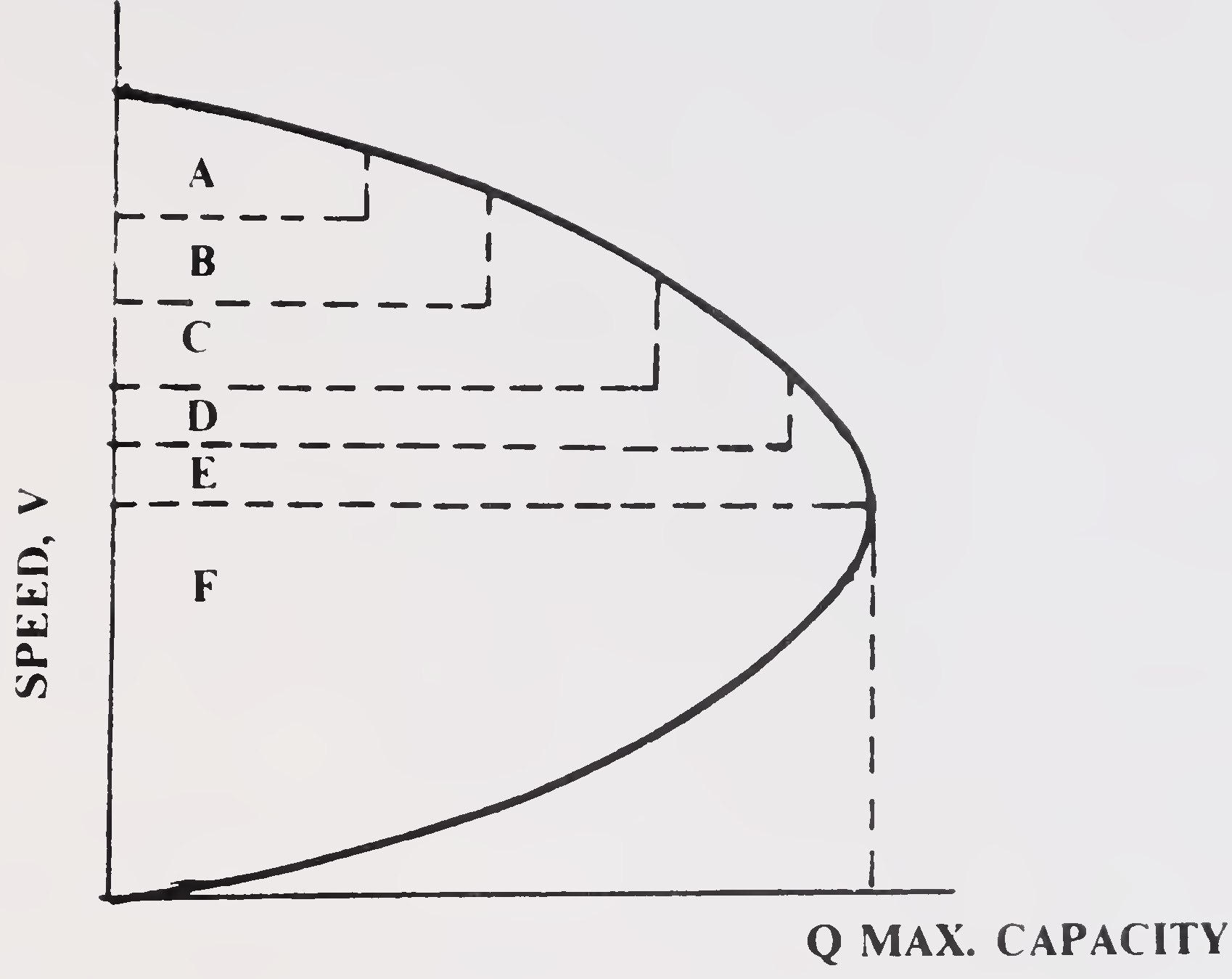
Fig. 2. Speed volume curve showing levels of service
| Level of Service A | : | Represents a condition of free flow. Individual users are virtually unaffected by the presence of others in the traffic stream. Freedom to select desired speeds and to manoeuvre within the traffic stream is high. The general level of comfort and convenience provided to the road users is excellent. |
| Level of Service B | : | Represents a zone of stable flow, with the drivers still having reasonable freedom to select their desired speed and manoeuvre within the traffic stream. Level of comfort and convenience provided is somewhat less than level of service A, because the presence of other vehicles in the traffic stream begins to affect individual behaviour. |
| Level of Service C | : | This also is a zone of stable flow, but marks the beginning of the range of flow in which the operation of individual users becomes significantly affected by interactions with others in the traffic stream. The selection of speed is now affected by the presence of others, and manoeuvring within the traffic stream requires substantial vigilance on the part of the user. The general level of comfort and convenience declines noticeably at this level.7 |
| Level of Service D | : | Represents the limit of stable flow, with conditions approaching close to unstable flow. Due to high density, the drivers are severely restricted in their freedom to select desired speed and manoeuvre within the traffic stream. The general level of comfort and convenience is poor. Small increases in traffic flow will usually cause operational problems at this level |
| Level of Service E | : | Represents operating conditions when traffic volumes are at or close to the capacity level. The speeds are reduced to a low, but relatively uniform value. Freedom to manoeuvre within the traffic stream is extremely difficult, and is generally accomplished by forcing a vehicle to give way to accommodate such manoeuvres. Comfort and convenience are extremely poor, and driver frustration is generally high. Operations at this level are usually unstable, because small increases in flow or minor disturbances within the traffic stream will cause breakdowns |
| Level of Service F | : | Represents zone of forced or breakdown flow. This condition occurs when the amount of traffic approaching a point exceeds the amount which can pass it Queues form behind such locations. Operations within the queue are characterised by stop-and-go waves, which are extremely unstable. Vehicles may progress at a reasonable speed for several hundred metres and may then be required to stop in a cyclic fashion. Due to high volumes, break-down occurs, and long queues and delays result |
From the viewpoint of smooth traffic flow, it is not advisable to design the width of road pavement for a traffic volume equal to its capacity which is available at LOS E. At this level, the speeds are low (typically half the free speed) and freedom to manoeuvre within the traffic stream is extremely restricted. Besides, at this level, even a small increase in volume would lead to forced flow situation and breakdowns within the traffic stream. Even the flow conditions at LOS C and D involve significant vehicle interaction leading to lower level of comfort and convenience. In contrast, Level of Service B represents a stable flow zone which affords reasonable freedom to drivers in terms of speed selection and manoeuvres within the traffic stream. Under normal circumstances, use of LOS B is considered adequate for the design of rural highways. At this level, volume of traffic will be around 0.5 times the maximum capacity and this is taken as the "design service volume" for the purpose of adopting design values. 8
It is recommended that on major arterial routes LOS B should be adopted for design purposes. On other roads under exceptional circumstances, LOS C could also be adopted for design. Under these conditions, traffic will experience congestion and inconvenience during some of the peak hours which may be acceptable. This is a planning decision which should be taken in each case specifically after carefully weighing all the related factors. For LOS C, design service volumes can be taken as 40 per cent higher than those for LOS B given in subsequent paragraphs.
In the context of rural highways, it is usual to adopt daily traffic volumes for design instead of hourly volumes. Therefore, the hourly flows need to be converted to daily values on the basis of observed or anticipated hourly pattern of traffic during the 24 hour day. Currently, the peak hour factor on trunk routes in the country is around 8-10 per cent of the AADT and the capacity figures recommended in the guidelines have been based on this.
The design service volume that should be considered for design/improvement of a road facility should be the expected volume at the end of the design life. This can be computed by projecting the present volume at an appropriate traffic growth rate. The traffic growth rate should be established after careful study of past trends and potential for future growth of the traffic.
The result of the presence of slow moving vehicles in traffic stream is that it affects the free flow of traffic. A way of accounting for the interaction of various kinds of vehicles is to express the capacity of roads in terms of a common unit. The unit generally employed is the passenger car unit'. Tentative equivalency factors for conversion of different types of vehicles into equivalent passenger car units based on their relative interference value, are given in Table 1. These factors are meant for open sections and should not be applied to road intersections. It needs to be recognised that the conversion factors are subject to variation dependent upon the composition of traffic, road geometrics and travel speeds. The equivalency factors given below are considered9
representative of the situations normally occurring and can therefore be adopted for general design purposes.
| S.No. | Vehicle Type | Equivalency Factor |
|---|---|---|
| Fast Vehicles | ||
| 1. | Motor Cycle or Scooter | 0.50 |
| 2. | Passenger Car, Pick-up Van or Auto-rickshaw | 1.00 |
| 3. | Agricultural Tractor, Light Commercial Vehicle | 1.50 |
| 4. | Truck or Bus | 3.00 |
| 5. | Truck-trailer, Agricultural Tractor-trailer | 4.50 |
| Slow Vehicles | ||
| 6. | Cycle | 0.50 |
| 7. | Cycle-rickshaw | 2.00 |
| 8. | Hand Cart | 3.00 |
| 9. | Horse-drawn vehicle | 4.00 |
| 10. | Bullock Cart* | 8.00 |
| * For smaller bullock-carts, a value of 6 will be appropriate. | ||
In practice, the equivalency factors will vary according to terrain. However, for purpose of these guidelines, the same equivalency factors as given above can be used for rolling/hilly sections since the effect of terrain has been accounted for in a consolidated manner in the Design Service Volumes recommended subsequently in Tables 2, 3 and 4 for different widths of road.
Single-lane bi-directional roads are of common occurrence in low volume corridors. For safe and smooth operation of traffic, a single lane road should have at least 3.75 metre wide paved carriageway with good quality shoulders such as moorum shoulders of minimum 1.0 metre width on either side.
The recommended design service volumes of single — lane roads are given in Table 2.10
| S. No. | Terrain | Curvature (Degrees per Kilometre) | Suggested Design Service Volume in PCU/day |
|---|---|---|---|
| 1. | Plain | Low (0-50) |
2000 |
|
High (above 51) |
1900 | ||
| 2. | Rolling | Low (0-100) |
1800 |
| High (above 101) |
1700 | ||
| 3. | Hilly | Low (0-200) |
1600 |
| High (above 201) |
1400 |
The above values are applicable for black-topped pavements. When the pavement is not black-topped, the design service volume will be lower by about 20-30 per cent.
In locations where only low quality shoulders are available (such as earthen shoulders made of plastic soil), the design service volumes should be taken as 50 per cent of the values given in Table 2.
Intermediate lane roads are those which have a pavement width of around 5.5 m with good usable shoulders on either side. The recommended design service volumes for these roads are given in Table 3.
Recommended design service volumes for two lane mads are given in Table 4.
The values recommended above are based on the assumptions that the road has a 7 m wide carriageway and good11
| S.N. | Terrain | Curvature (Degrees per Kilometre) | Design Service Volume in PCU/day |
|---|---|---|---|
| 1. | Plain |
Low (0-50) | 6,000 |
|
High (above 51) | 5,800 | ||
| 2. | Rolling |
Low (0-100) | 5,700 |
|
High (above 101) | 5,600 | ||
| 3. | Hilly |
Low (0-200) | 5,200 |
|
High (above 201) | 4,500 |
| S.N. | Terrain | Curvature (Degrees per Kilometre) | Design Service Volume in PCU/day |
|---|---|---|---|
| 1. | Plain |
Low (0-50) | 15,000 |
|
High (above 51) | 12,500 | ||
| 2. | Rolling |
Low (0-100) | 11,000 |
|
High (above 101) | 10,000 | ||
| 3. | Hilly |
Low (0-200) | 7,000 |
|
High (above 201) | 5,00012 |
earthen shoulders are available. The capacity figures relate to peak hour traffic in the range of 8-10 per cent and LOS B.
The capacity of two lane roads can be increased by providing paved and surfaced shoulders of at least 1.5 metre width on either side. Provision of hard shoulders results in slow moving traffic being able to travel on the shoulder which reduces the interference to fast traffic on the main carriageway. Under these circumstances, 15 per cent increase in capacity can be expected vis-a-vis the values given in Table 4.
Where shoulder width or carriageway width on a two lane road are restricted, there will be a certain reduction in capacity. Table 5 gives the recommended reduction factors on this account over the capacity values given in Table 4.
|
Usable* shoulder width (m) |
3.50 m lane | 3.25 m lane | 3.00 m lane |
|---|---|---|---|
| > 1.8 | 1.00 | 0 92 | 0.84 |
| 1.2 | 0.92 | 0.85 | 0.77 |
| 0.6 | 0.81 | 0.75 | 0.68 |
| 0 | 0.70 | 0.64 | 0.58 |
| * Usable shoulder width refers to well-maintained earth/moorum gravel shoulder-which can safely permit occasional passage of vehicles. | |||
Sufficient information about the capacity of multi-lane roads under mixed traffic conditions is not yet available. Capacity on dual carriageway roads can also be affected by factors like kerb shyness on the median side vehicle parking etc. Tentatively, a value of 35,000 PCUs can be adopted for four-lane divided carriageways located in plain terrain. It is assumed for this purpose that reasonable good earthen shoulders exist on the outer side, and a minimum 3.0 m wide central verge exists.
Provision of hard shoulders on dual carriageways can further increase the capacity as explained in para 10.3. In case well13
designed paved shoulders of 1.5 metre width are provided, the capacity value of four-lane dual roads can he taken up to 40,000 PCUs.
The capacity values mentioned above relate to LOS B On dual carriageways it will normally not be desirable to adopt LOS C.14